Visual inspection of signals • ninetails

Note: Signal visualization functions are available for both the Guppy legacy pipeline (fast5-based: plot_squiggle_fast5(), plot_tail_range_fast5()) and the Dorado DRS pipeline (POD5-based: plot_squiggle_pod5(), plot_tail_range_pod5()).

This vignette describes functions for visual inspection of raw nanopore signals. For interactive signal browsing with filters and read navigation, see the Signal Viewer tab in the Shiny dashboard: vignette("shiny_app").

Plotting whole reads

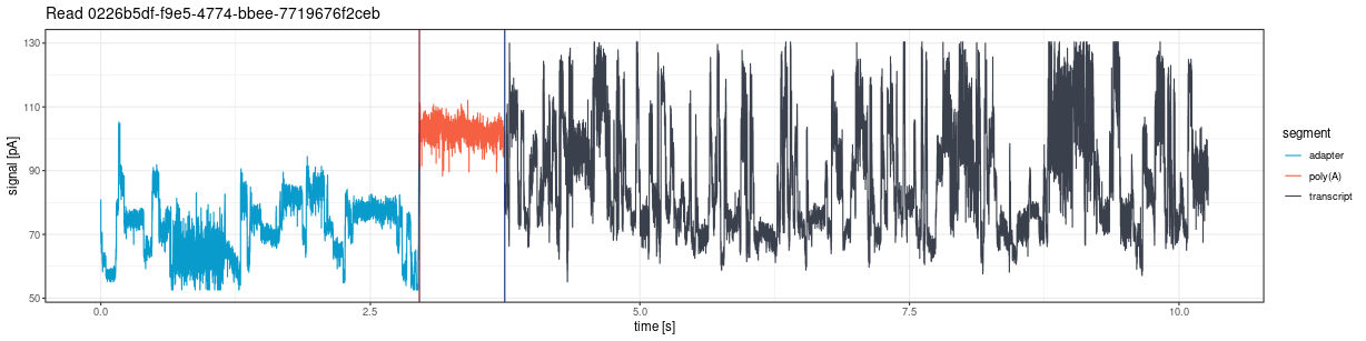
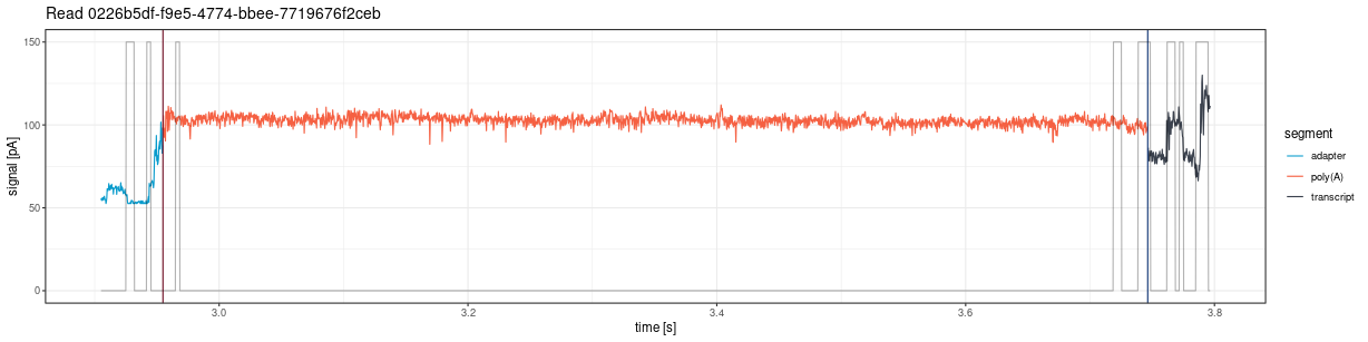
plot_squiggle_fast5()

Draw the entire signal (squiggle) for a given read from fast5 files:

plot <- ninetails::plot_squiggle_fast5(
  readname = "0226b5df-f9e5-4774-bbee-7719676f2ceb",
  nanopolish = system.file('extdata', 'test_data',
                           'nanopolish_output.tsv',
                           package = 'ninetails'),
  sequencing_summary = system.file('extdata', 'test_data',
                                   'sequencing_summary.txt',
                                   package = 'ninetails'),
  workspace = system.file('extdata', 'test_data',
                          'basecalled_fast5',
                          package = 'ninetails'),
  basecall_group = 'Basecall_1D_000',
  moves = FALSE,
  rescale = TRUE
)
print(plot)

Parameters

Parameter	Type	Default	Description
`readname`	character	required	Unique read identifier
`nanopolish`	character/data.frame	required	Path to Nanopolish polya output or a pre-loaded data frame
`sequencing_summary`	character/data.frame	required	Path to sequencing summary or a pre-loaded data frame
`workspace`	character	required	Path to directory with multi-fast5 files
`basecall_group`	character	`"Basecall_1D_000"`	Fast5 hierarchy level for basecall data
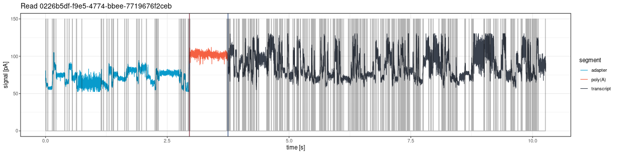
`moves`	logical	`FALSE`	If `TRUE`, show move transitions as background shading
`rescale`	logical	`TRUE`	If `TRUE`, scale signal to picoamperes (pA) per second

The plot shows vertical lines marking poly(A) tail boundaries:

Red: 5’ end (poly(A) start)
Navy blue: 3’ end (poly(A) end)

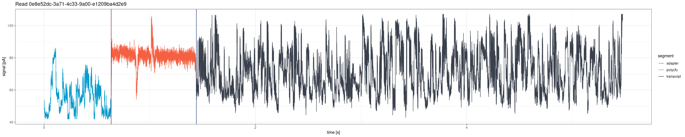
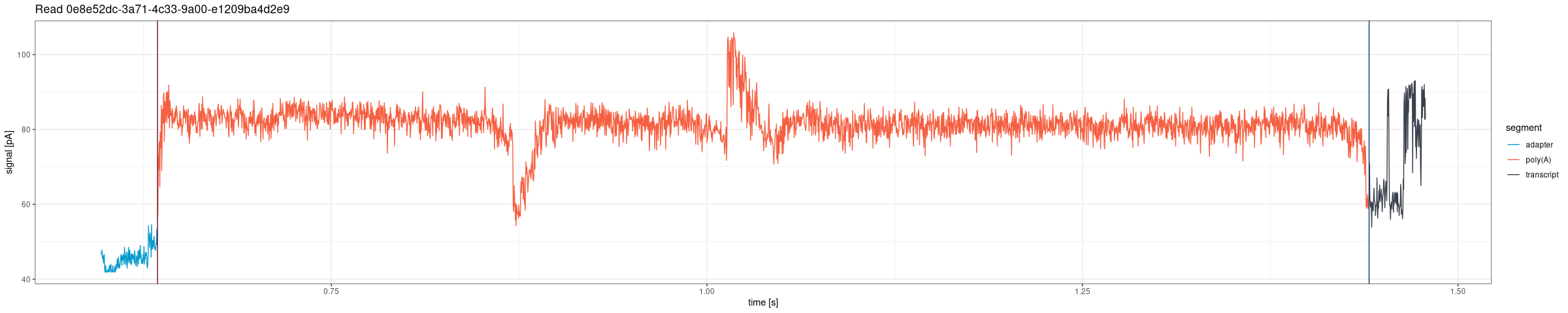
Signal plotted with moves=FALSE Signal plotted with moves=TRUE

plot_squiggle_pod5()

Draw the entire signal for a given read from POD5 files (Dorado DRS pipeline):

plot <- ninetails::plot_squiggle_pod5(
  readname = "0e8e52dc-3a71-4c33-9a00-e1209ba4d2e9",
  dorado_summary = system.file('extdata', 'test_data', 'pod5_DRS',
                               'aligned_summary.txt',
                               package = 'ninetails'),
  workspace = system.file('extdata', 'test_data', 'pod5_DRS',
                          package = 'ninetails'),
  rescale = TRUE
)
print(plot)

Parameters

Parameter	Type	Default	Description
`readname`	character	required	Unique read identifier
`dorado_summary`	character/data.frame	required	Path to Dorado summary file or a pre-loaded data frame with `read_id`, `poly_tail_start`, `poly_tail_end`, and `filename` columns
`workspace`	character	required	Path to directory containing POD5 files
`rescale`	logical	`TRUE`	If `TRUE`, scale signal to picoamperes (pA)
`residue_data`	data.frame	`NULL`	Non-A residue table for overlay highlighting (optional)
`nonA_flank`	numeric	`250`	Number of raw signal positions flanking each non-A overlay rectangle

Note: The moves parameter is not available for POD5-based functions. Move data is not stored in POD5 files in a format accessible without the Dorado basecaller internals.

Full read signal from POD5, rescaled to pA

Plotting tail range

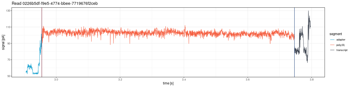
plot_tail_range_fast5()

Plot only the poly(A) tail region from fast5 files, with optional flanking sequence:

plot <- ninetails::plot_tail_range_fast5(
  readname = "0226b5df-f9e5-4774-bbee-7719676f2ceb",
  nanopolish = system.file('extdata', 'test_data',
                           'nanopolish_output.tsv',
                           package = 'ninetails'),
  sequencing_summary = system.file('extdata', 'test_data',
                                   'sequencing_summary.txt',
                                   package = 'ninetails'),
  workspace = system.file('extdata', 'test_data',
                          'basecalled_fast5',
                          package = 'ninetails'),
  basecall_group = 'Basecall_1D_000',
  moves = TRUE,
  rescale = TRUE
)
print(plot)

Accepts the same parameters as plot_squiggle_fast5().

Tail region plotted with moves=FALSE

plot_tail_range_pod5()

Plot only the poly(A) tail region from POD5 files, with configurable flanking and optional non-A residue overlay:

plot <- ninetails::plot_tail_range_pod5(
  readname = "0e8e52dc-3a71-4c33-9a00-e1209ba4d2e9",
  dorado_summary = system.file('extdata', 'test_data', 'pod5_DRS',
                               'aligned_summary.txt',
                               package = 'ninetails'),
  workspace = system.file('extdata', 'test_data', 'pod5_DRS',
                          package = 'ninetails'),
  flank = 150,
  rescale = TRUE
)
print(plot)

Parameters

Parameter	Type	Default	Description
`readname`	character	required	Unique read identifier
`dorado_summary`	character/data.frame	required	Path to Dorado summary file or pre-loaded data frame
`workspace`	character	required	Path to directory containing POD5 files
`flank`	numeric	`150`	Number of raw signal positions to include on each side of the poly(A) region
`rescale`	logical	`TRUE`	If `TRUE`, scale signal to picoamperes (pA)
`residue_data`	data.frame	`NULL`	Non-A residue table for overlay highlighting (optional)
`nonA_flank`	numeric	`250`	Width (in raw positions) of each non-A overlay rectangle

Poly(A) tail region from POD5, rescaled to pA

Non-A residue overlay

When residue_data is provided, both plot_squiggle_pod5() and plot_tail_range_pod5() overlay semi-transparent rectangles at the estimated positions of detected non-adenosine residues. Each rectangle is colored by residue type:

Residue	Color	Hex
C (cytidine)	Dark gray	`#3a424f`
G (guanosine)	Green	`#50a675`
U (uridine)	Light blue-gray	`#b0bdd4`

The nonA_flank parameter controls the width of each rectangle in raw signal positions (default: 250 positions on each side of the estimated center). A letter label (C, G, or U) is placed at the top of each rectangle.

# Plot with non-A overlay
plot <- ninetails::plot_tail_range_pod5(
  readname       = "0e8e52dc-3a71-4c33-9a00-e1209ba4d2e9",
  dorado_summary = dorado_summary_df,
  workspace      = "/path/to/pod5/",
  flank          = 150,
  rescale        = FALSE,
  residue_data   = residue_data,
  nonA_flank     = 250
)
print(plot)

Position conversion: the function converts est_nonA_pos (nucleotide position from the 3’ end) to raw signal coordinates using linear interpolation between poly_tail_start and poly_tail_end.

Plotting tail segments

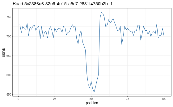
plot_tail_chunk()

Visualize a specific signal chunk from the segmentation step. This function is mainly useful for debugging the pipeline or understanding how individual segments are classified.

# First, create tail chunk list using pipeline functions
tfl <- ninetails::create_tail_feature_list(...)
tcl <- ninetails::create_tail_chunk_list(tail_feature_list = tfl, num_cores = 2)

# Then plot a specific chunk
plot <- ninetails::plot_tail_chunk(
  chunk_name = "5c2386e6-32e9-4e15-a5c7-2831f4750b2b_1",
  tail_chunk_list = tcl
)
print(plot)

Parameters

Parameter	Type	Description
`chunk_name`	character	Identifier of the chunk (format: `readname_chunkindex`)
`tail_chunk_list`	list	Output from `create_tail_chunk_list()`

Note: This function shows raw signal only; no scaling to picoamperes is applied.

Selected tail chunk

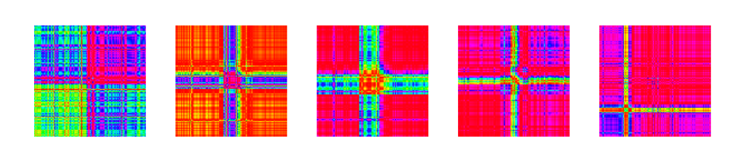
Plotting Gramian Angular Fields

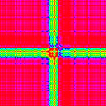
plot_gaf()

Visualize a single GAF matrix used for CNN classification. Each GAF image has two channels representing the Gramian Angular Summation Field (GASF) and the Gramian Angular Difference Field (GADF).

# First, create GAF list using pipeline functions
gl <- ninetails::create_gaf_list(tail_chunk_list = tcl, num_cores = 2)

# Plot a specific GAF
plot <- ninetails::plot_gaf(
  gaf_name = "5c2386e6-32e9-4e15-a5c7-2831f4750b2b_1",
  gaf_list = gl
)
print(plot)

Parameters

Parameter	Type	Description
`gaf_name`	character	Identifier of the GAF (same format as chunk names)
`gaf_list`	list	Output from `create_gaf_list()`

Gramian angular field

plot_multiple_gaf()

Plot all GAFs in a list. Each plot is saved as an image file in the working directory.

ninetails::plot_multiple_gaf(
  gaf_list  = gl,
  num_cores = 10
)

Parameters

Parameter	Type	Default	Description
`gaf_list`	list	required	Output from `create_gaf_list()`
`num_cores`	integer	`1`	Number of cores for parallel rendering

Warning: Use with caution. GAF lists can be very large, and plotting all at once may overload the system.

Multiple Gramian angular fields

Signal visualization options

Option	Description	Applies to
`rescale = FALSE`	Raw signal per position	Fast5, POD5
`rescale = TRUE`	Signal scaled to picoamperes (pA) per second	Fast5, POD5
`moves = FALSE`	Signal only	Fast5 only
`moves = TRUE`	Signal with move transitions in background	Fast5 only
`flank`	Positions flanking tail region (default: 150)	POD5 tail range only
`residue_data`	Non-A residue overlay highlighting	POD5 only
`nonA_flank`	Width of overlay rectangles (default: 250)	POD5 only

Use cases

Signal visualization is useful for:

Quality control: Inspect individual reads for signal quality and verify that poly(A) boundaries are correctly identified
Debugging: Understand why specific reads were classified incorrectly by examining the raw signal shape
Validation: Verify that detected non-adenosines correspond to visible signal deviations within the poly(A) region
Publication figures: Generate high-quality signal plots for manuscripts and presentations
Non-A overlay inspection: Confirm that the residue position estimates align with actual signal perturbations

Interactive signal viewer

For browsing signals interactively with filters, read navigation, and non-A overlay, use the Shiny dashboard’s Signal Viewer tab:

ninetails::launch_signal_browser(
  summary_file = "/path/to/dorado_summary.txt",
  pod5_dir     = "/path/to/pod5/",
  residue_file = "/path/to/nonadenosine_residues.txt"
)

The dashboard provides:

Filterable read list (by poly(A) length, decoration status, residue type, alignment genome, mapping quality)
Previous/Next navigation through filtered reads
Static Viewer sub-tab with full signal and zoomed poly(A) region
Dynamic Explorer sub-tab with interactive Plotly zoom and pan
Automatic non-A residue overlay when residue data is available

See vignette("shiny_app") for complete documentation.

Summary of signal inspection functions

Function	Description	Input
`plot_squiggle_fast5()`	Full read signal	Fast5 files
`plot_squiggle_pod5()`	Full read signal (+ optional non-A overlay)	POD5 files
`plot_tail_range_fast5()`	Poly(A) tail signal only	Fast5 files
`plot_tail_range_pod5()`	Poly(A) tail signal (+ optional non-A overlay)	POD5 files
`plot_tail_chunk()`	Signal segment from segmentation	Intermediate data
`plot_gaf()`	Single GAF image (GASF + GADF)	Intermediate data
`plot_multiple_gaf()`	Batch GAF rendering	Intermediate data