This vignette documents all plotting functions provided by
ninetails for visualizing classification results,
residue composition, poly(A) tail distributions, and positional
patterns. For interactive exploration of these plots, see
vignette("shiny_app").
All plotting functions return ggplot2 objects and can be
further customized with standard ggplot2 layers (themes, scales,
labels).
Read classification
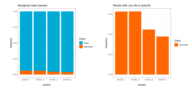
plot_class_counts() produces bar charts of read
classification results. The type argument controls the
level of detail.
plt <- ninetails::plot_class_counts(
  class_data       = class_data,
  grouping_factor  = "sample_name",
  frequency        = TRUE,
  type             = "N"
)
print(plt)
Parameters
| Parameter | Type | Default | Description |
|---|---|---|---|
class_data |
data.frame | required | Read classification table from ninetails |
grouping_factor |
character | NA |
Column name to group by (e.g., "sample_name",
"group") |
frequency |
logical | FALSE |
If TRUE, show proportions instead of raw counts |
type |
character | "N" |
Level of detail (see below) |
Classification views
| Type | Description | Categories shown |
|---|---|---|
"N" |
Summary | decorated, blank, unclassified |
"R" |
Detailed | All comment codes (YAY, MAU, MPU, IRL, UNM, BAC) |
"A" |
Decorated only | Only decorated reads |
Detailed classification
All reads — decorated, blank, and unclassified — are included and colour-coded by their comment code.
plt <- ninetails::plot_class_counts(
  class_data       = class_data,
  grouping_factor  = "sample_name",
  frequency        = TRUE,
  type             = "R"
)
print(plt)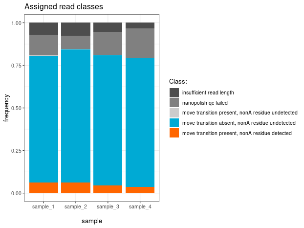
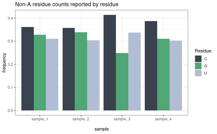
Residue counts
plot_residue_counts() shows the distribution of
non-adenosine residue types (C, G, U) across samples or conditions. Two
counting modes are available:
- By residue (default): Counts every individual non-A residue occurrence. A read with two C residues contributes 2 to the C count.
-
By read (
by_read = TRUE): Counts each read once per residue type. A read with two C residues contributes 1 to the C count.
plt <- ninetails::plot_residue_counts(
  residue_data     = residue_data,
  grouping_factor  = "sample_name",
  frequency        = TRUE,
  by_read          = FALSE
)
print(plt)
Parameters
| Parameter | Type | Default | Description |
|---|---|---|---|
residue_data |
data.frame | required | Non-A residue table from ninetails |
grouping_factor |
character | NA |
Grouping column |
frequency |
logical | FALSE |
Show proportions instead of counts |
by_read |
logical | FALSE |
Count by read instead of by individual residue |
Non-A abundance
plot_nonA_abundance() shows the frequency of reads
containing one, two, or three or more separate non-adenosine residues
per read. Frequencies are computed relative to the total number of
decorated reads in each sample.
plt <- ninetails::plot_nonA_abundance(
  residue_data     = residue_data,
  grouping_factor  = "sample_name"
)
print(plt)Poly(A) tail length distribution
plot_tail_distribution() plots density distributions of
poly(A) tail lengths across samples or conditions. Central tendency
lines can be overlaid.
plt <- ninetails::plot_tail_distribution(
  input_data       = class_data,
  grouping_factor  = "sample_name",
  max_length       = 200,
  value_to_show    = "median",
  ndensity         = TRUE
)
print(plt)
Parameters
| Parameter | Type | Default | Description |
|---|---|---|---|
input_data |
data.frame | required | Data frame with polya_length column (class data or
merged table) |
grouping_factor |
character | NA |
Grouping column |
max_length |
numeric | 200 |
Upper limit of the x-axis |
value_to_show |
character | NA |
Central tendency line: "mean", "median",
"mode", or NA (none) |
ndensity |
logical | TRUE |
If TRUE, normalize density so the peak equals 1 across
groups |
Custom color palettes can be applied:
# Apply a custom palette
plt + ggplot2::scale_color_manual(
  values = c("#D7191C", "#2C7BB6", "#FDAE61", "#ABD9E9")
)
Non-A position distribution (rug density)
plot_rug_density() visualizes the positional
distribution of non-adenosine residues along poly(A) tails. Each point
represents one detected modification, plotted against its estimated
position from the 3’ end (x-axis) and the total tail length of the read
(y-axis). Marginal density curves on both axes show the overall
distribution shape. Call the function once per nucleotide type.
plt_C <- ninetails::plot_rug_density(
  residue_data = residue_data,
  base         = "C",
  max_length   = 100
)
print(plt_C)
Parameters
| Parameter | Type | Default | Description |
|---|---|---|---|
residue_data |
data.frame | required | Non-A residue table |
base |
character | required | Nucleotide type: "C", "G", or
"U"
|
max_length |
numeric | required | Maximum tail length for axis limits |
Note: This function requires the
cowplotpackage. Install withinstall.packages("cowplot").
For large datasets, consider subsampling before plotting to keep the scatter readable:
# Subsample to 1000 points per base type
set.seed(42)
rd_sub <- residue_data[residue_data$prediction == "C", ]
if (nrow(rd_sub) > 1000) {
  keep <- sample.int(nrow(rd_sub), 1000, replace = FALSE)
  rd_sub <- rd_sub[keep, ]
}
plt <- ninetails::plot_rug_density(rd_sub, base = "C", max_length = 200)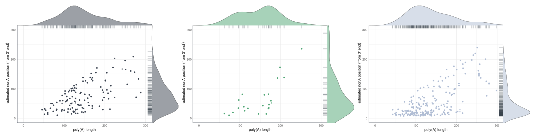
Panel characteristics
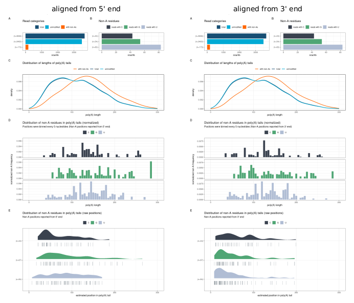
plot_panel_characteristics() produces a multi-panel
summary of the full tail composition for a dataset or subset (e.g., a
single sample, group, or transcript). The resulting plot can be aligned
from either the 5’ or 3’ end of the tail.
plt <- ninetails::plot_panel_characteristics(
  input_residue_data            = residue_data,
  input_class_data              = class_data,
  input_merged_nonA_tables_data = NULL,
  type                          = "default",
  max_length                    = 100,
  direction_5_prime             = TRUE
)
print(plt)
Parameters
| Parameter | Type | Default | Description |
|---|---|---|---|
input_residue_data |
data.frame | required | Non-A residue table |
input_class_data |
data.frame | required | Read classification table |
input_merged_nonA_tables_data |
data.frame | NULL |
Merged table (optional) |
type |
character | "default" |
Panel layout type |
max_length |
numeric | 100 |
Maximum tail length |
direction_5_prime |
logical | TRUE |
Align from 5’ end (TRUE) or 3’ end
(FALSE) |
The panel contains the following subplots:
- A — Read counts
- B — Frequency of non-adenosine residues
- C — Poly(A) tail length distribution
- D — Normalised distribution of non-adenosines (binned by length)
- E — Raw distribution of non-adenosines
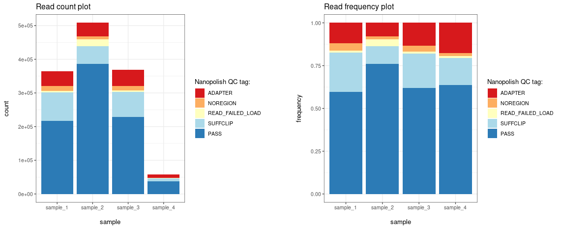
Nanopolish QC tags
Note: This section applies only to the Guppy legacy pipeline (
check_tails_guppy()).
The nanopolish_qc() and
plot_nanopolish_qc() functions allow visualization of QC
tags assigned by the Nanopolish polya function.
# Summarise QC tags per sample
qc_summary <- ninetails::nanopolish_qc(
  class_data,
  grouping_factor = "sample_name"
)

# Plot by read count
plt_count <- ninetails::plot_nanopolish_qc(qc_summary, frequency = FALSE)

# Plot by frequency
plt_freq <- ninetails::plot_nanopolish_qc(qc_summary, frequency = TRUE)

print(plt_count)
print(plt_freq)
Parameters (nanopolish_qc)
| Parameter | Type | Default | Description |
|---|---|---|---|
class_data |
data.frame | required | Read classification table |
grouping_factor |
character | NA |
Grouping column |
Parameters (plot_nanopolish_qc)
| Parameter | Type | Default | Description |
|---|---|---|---|
processing_info |
data.frame | required | Output from nanopolish_qc()
|
frequency |
logical | FALSE |
Show proportions instead of counts |
Interactive dashboard
For interactive exploration of all plots described above, ninetails
provides a Shiny dashboard. See vignette("shiny_app") for
details.
ninetails::launch_signal_browser(
  class_file   = "/path/to/read_classes.txt",
  residue_file = "/path/to/nonadenosine_residues.txt"
)
Summary of plotting functions
| Function | Description | Required data |
|---|---|---|
plot_class_counts() |
Read classification bar chart | class_data |
plot_residue_counts() |
Residue type distribution (C/G/U) | residue_data |
plot_nonA_abundance() |
Reads with 1, 2, 3+ non-A residues | residue_data |
plot_tail_distribution() |
Poly(A) tail length density |
class_data or merged table |
plot_rug_density() |
Non-A position scatterplot with density | residue_data |
plot_panel_characteristics() |
Multi-panel composition summary |
class_data + residue_data
|
plot_nanopolish_qc() |
Nanopolish QC tag distribution |
nanopolish_qc() output |
plot_squiggle_fast5() |
Full read signal (fast5) | Fast5 files |
plot_squiggle_pod5() |
Full read signal (POD5) | POD5 files |
plot_tail_range_fast5() |
Poly(A) tail signal (fast5) | Fast5 files |
plot_tail_range_pod5() |
Poly(A) tail signal (POD5) | POD5 files |
plot_tail_chunk() |
Signal segment | Intermediate data |
plot_gaf() / plot_multiple_gaf()
|
Gramian Angular Fields | Intermediate data |